Data types
Day 2, Session 7
Data types
Strings, factors and dates


1.
Strings
The stringr package is your tidyverse companion to all things strings.
stringr provides a cohesive set of functions that make working with character data in R as easy as possible. Most any task you can think of that involves character data can be accomplished with stringr.
It's part of the core tidyverse, along with packages like dplyr and ggplot2, so stringr functions play really nicely with dplyr functions like filter() and mutate().
Let's look at a concrete example.
Breed Traits data set
breed_traits## # A tibble: 195 × 15## breed affection shedding drooling openness playfulness protectiveness## <chr> <dbl> <dbl> <dbl> <dbl> <dbl> <dbl>## 1 Retrievers (L… 5 4 2 5 5 3## 2 French Bulldo… 5 3 3 5 5 3## 3 German Shephe… 5 4 2 3 4 5## 4 Retrievers (G… 5 4 2 5 4 3## 5 Bulldogs 4 3 3 4 4 3## 6 Poodles 5 1 1 5 5 5## # ℹ 189 more rows## # ℹ 8 more variables: adaptability <dbl>, trainability <dbl>, energy <dbl>,## # barking <dbl>, stimulation_needs <dbl>, good_w_children <dbl>,## # good_w_other_dogs <dbl>, grooming_freq <dbl>The breed_traits dataset is a fun dataset that contains information on 195 dog breeds, with scores (on a 1-5 scale) for 15 traits (e.g. how affectionate the breed is, how much it sheds, how playful it is, etc). This data comes courtesy of the American Kennel Club.
In our analysis, want to compare traits across terrier breeds only, of which there are many types.
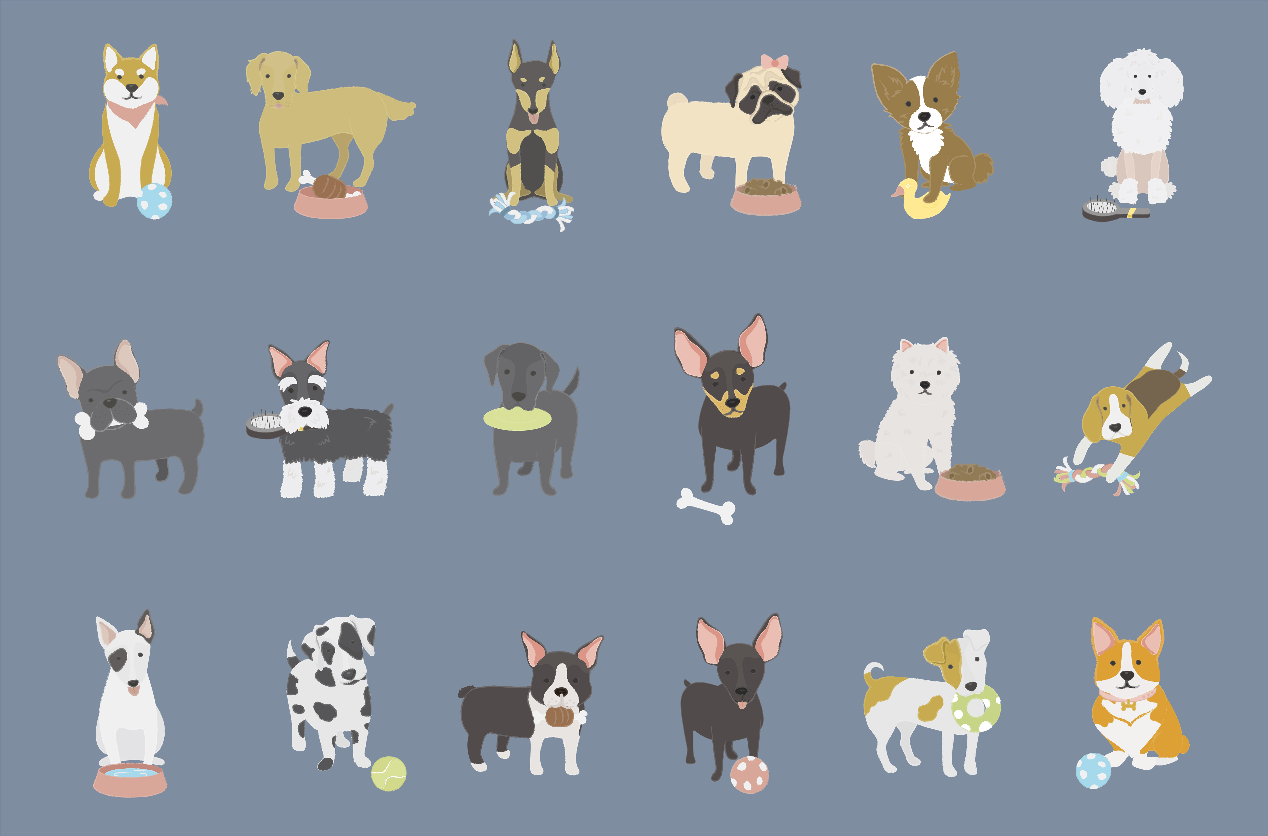
To make this very clear, we have 195 dog breeds (with 18 very good boys and girls are pictured here as an example)...
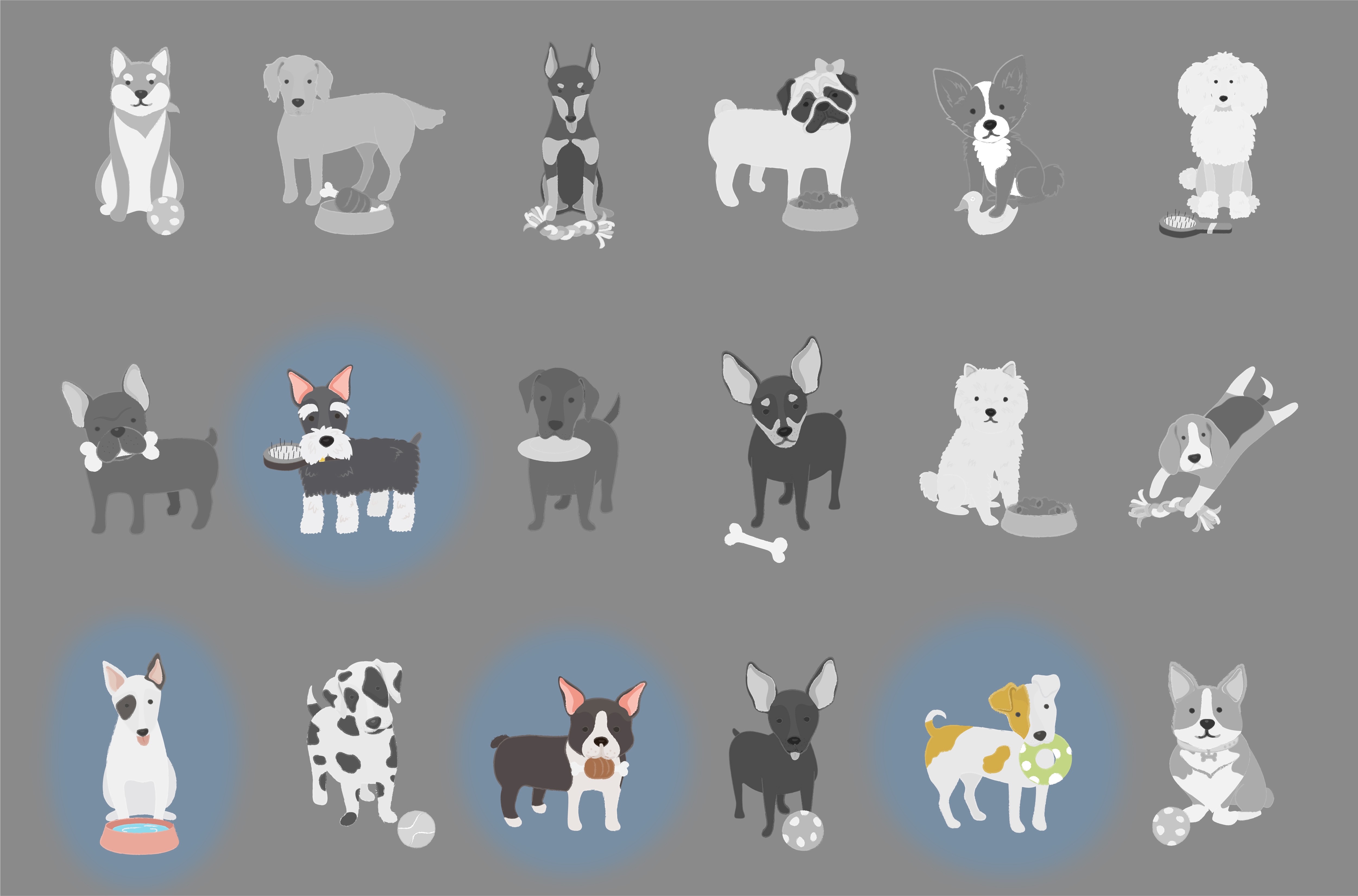
...and we want to subset the data so that we can continue our analysis on terrier breeds. Note that I don't know how many of the 195 breeds in the dataset have "terrier" as part of their name, but I want to keep them all.
(The four highlighted breeds, from top to bottom, left to right, are Scottish, Bull, Boston, and Russell terriers.)
Sniffing out terrier breeds
breed_traits %>% filter(breed == "Yorkshire Terriers")## # A tibble: 1 × 15## breed affection shedding drooling openness playfulness protectiveness## <chr> <dbl> <dbl> <dbl> <dbl> <dbl> <dbl>## 1 Yorkshire Ter… 5 1 1 5 4 5## # ℹ 8 more variables: adaptability <dbl>, trainability <dbl>, energy <dbl>,## # barking <dbl>, stimulation_needs <dbl>, good_w_children <dbl>,## # good_w_other_dogs <dbl>, grooming_freq <dbl>When I say "subset", alarm bells are probably going off in your head that we we'll be using the filter() function.
Using what we've already know how to do, we can print the breed_traits table and scan through the paginated results in RMarkdown to find our first match — Yorkshire terriers.
We'll use the == operator to match the string, and get one row in the output.
Sniffing out terrier breeds
breed_traits %>% filter(breed %in% c("Yorkshire Terriers", "Boston Terriers"))## # A tibble: 2 × 15## breed affection shedding drooling openness playfulness protectiveness## <chr> <dbl> <dbl> <dbl> <dbl> <dbl> <dbl>## 1 Yorkshire Ter… 5 1 1 5 4 5## 2 Boston Terrie… 5 2 1 5 5 3## # ℹ 8 more variables: adaptability <dbl>, trainability <dbl>, energy <dbl>,## # barking <dbl>, stimulation_needs <dbl>, good_w_children <dbl>,## # good_w_other_dogs <dbl>, grooming_freq <dbl>And then our second match — Boston terriers.
This time, we'll use the %in% operator to match a vector of strings, and get two rows in the output.
You can where this is going...
Sniffing out terrier breeds
breed_traits %>%
  filter(breed %in% c(
    "Yorkshire Terriers",
    "Boston Terriers",
    "West Highland White Terriers",
    "Scottish Terriers",
    "Fox Terriers (Wire)",
    ...
  )
)
If you think about extending this process to all 200 or so rows, you'll realize that filtering with explicit strings isn't really a scalable solution. Even in this relatively small and tidy dataset, we can see that it becomes tedious and error-prone very quickly.
Sniffing out terrier breeds
breed_traits %>%
  filter(breed %in% c(
    "Yorkshire Terriers",
    "Boston Terriers",
    "West Highland White Terriers",
    "Scottish Terriers",
    "Fox Terriers (Wire)",
    ...
  )
)
And you'd be right to intuit that there's a simpler way. All we, the humans, are doing is looking for the sequence "Terrier" in the breed column. This is exactly the kind of simple but highly repetitive task that's well-suited to outsource to our computers.
That's where stringr comes in.
Filtering with str_detect()
breed_traits %>% filter(str_detect(breed, "Terrier"))## # A tibble: 36 × 15## breed affection shedding drooling openness playfulness protectiveness## <chr> <dbl> <dbl> <dbl> <dbl> <dbl> <dbl>## 1 Yorkshire Te… 5 1 1 5 4 5## 2 Boston Terri… 5 2 1 5 5 3## 3 West Highlan… 5 3 1 4 5 5## 4 Scottish Ter… 5 2 2 3 4 5## 5 Soft Coated … 5 1 2 3 3 3## 6 Airedale Ter… 3 1 1 3 3 5## 7 Bull Terriers 4 3 1 4 4 3## 8 Russell Terr… 5 3 1 5 5 4## 9 Cairn Terrie… 4 2 1 3 4 4## 10 Staffordshir… 5 2 3 4 4 5## # ℹ 26 more rows## # ℹ 8 more variables: adaptability <dbl>, trainability <dbl>, energy <dbl>,## # barking <dbl>, stimulation_needs <dbl>, good_w_children <dbl>,## # good_w_other_dogs <dbl>, grooming_freq <dbl>The str_detect() function searches for the presence of a pattern in a string and returns a logical vector that's TRUE if the pattern is detected, or FALSE if it's not. That makes it a very powerful function in combination with filter().
In the example code, we keep only the rows where the sequence "Terrier" is found in the breed column, and drop the rest.
stringr functions
Character manipulation
str_sub("Introduction to the tidyverse", 21, 24)## [1] "tidy"We can extract (and replace) substrings from a vector using str_sub(), in this case by extracting the 21st through 24th characters which form the word "tidy".
stringr functions
Whitespace tools
str_trim(" Introduction to the tidyverse ")## [1] "Introduction to the tidyverse"We can trim whitespace from a string using str_trim(), which can be a quick and easy data cleaning step.
stringr functions
Locale-sensitive operations
str_to_upper("Introduction to the tidyverse")## [1] "INTRODUCTION TO THE TIDYVERSE"We can turn convert cases with str_to_upper() and turn strings into yells.
These functions are called "locale-sensitive operations" because they can follow capitalization and alphabetization rules in different languages.
stringr functions
Pattern matching
str_view_all("Introduction to the tidyverse", "[aeiou]")Introduction to the tidyverse
And we can visualize how patterns match to our data with str_view() (and str_view_all()). In this case, I'm looking to highlight the vowels in my input string, but the patterns you search for can be very flexible and powerful.
You may have noticed an elegant detail: all stringr functions start with the prefix "str_". This is especially nice when you're working in RStudio because typing that prefix out will trigger autocomplete and allow you to see all of the functions.
Your Turn 1
Use the str_subset() function to subset the elements of the fruit vector that are made up of two or more words.
# preview `fruit`, which is loaded along with stringrlibrary(stringr)fruit## [1] "apple" "apricot" "avocado" ## [4] "banana" "bell pepper" "bilberry" ## [7] "blackberry" "blackcurrant" "blood orange" ## [10] "blueberry" "boysenberry" "breadfruit" ## [13] "canary melon" "cantaloupe" "cherimoya" ## [16] "cherry" "chili pepper" "clementine" ## [19] "cloudberry" "coconut" "cranberry" ## [22] "cucumber" "currant" "damson" ## [25] "date" "dragonfruit" "durian" ## [28] "eggplant" "elderberry" "feijoa" ## [31] "fig" "goji berry" "gooseberry" ## [34] "grape" "grapefruit" "guava" ## [37] "honeydew" "huckleberry" "jackfruit" ## [40] "jambul" "jujube" "kiwi fruit" ## [43] "kumquat" "lemon" "lime" ## [46] "loquat" "lychee" "mandarine" ## [49] "mango" "mulberry" "nectarine" ## [52] "nut" "olive" "orange" ## [55] "pamelo" "papaya" "passionfruit" ## [58] "peach" "pear" "persimmon" ## [61] "physalis" "pineapple" "plum" ## [64] "pomegranate" "pomelo" "purple mangosteen"## [67] "quince" "raisin" "rambutan" ## [70] "raspberry" "redcurrant" "rock melon" ## [73] "salal berry" "satsuma" "star fruit" ## [76] "strawberry" "tamarillo" "tangerine" ## [79] "ugli fruit" "watermelon"We're looking for fruits like "bell pepper", "blood orange", etc.
Hint: Look up the help page for str_subset()
Hint: What character indicates that a string contains more than one word?
Solution: str_subset(fruit, " ")
Your Turn 1 Solution
Use a stringr function to subset the elements of the fruit vector that are made up of two or more words.
str_subset(fruit, " ")## [1] "bell pepper" "blood orange" "canary melon" ## [4] "chili pepper" "goji berry" "kiwi fruit" ## [7] "purple mangosteen" "rock melon" "salal berry" ## [10] "star fruit" "ugli fruit"2.
Factors
Categorical data in R are called "factors"
Each category is called a "level"
General Social Survey data set
library(forcats)gss_cat## # A tibble: 21,483 × 9## year marital age race rincome partyid relig denom tvhours## <int> <fct> <int> <fct> <fct> <fct> <fct> <fct> <int>## 1 2000 Never married 26 White $8000 to 9999 Ind,near r… Prot… Sout… 12## 2 2000 Divorced 48 White $8000 to 9999 Not str re… Prot… Bapt… NA## 3 2000 Widowed 67 White Not applicable Independent Prot… No d… 2## 4 2000 Never married 39 White Not applicable Ind,near r… Orth… Not … 4## 5 2000 Divorced 25 White Not applicable Not str de… None Not … 1## 6 2000 Married 25 White $20000 - 24999 Strong dem… Prot… Sout… NA## 7 2000 Never married 36 White $25000 or more Not str re… Chri… Not … 3## 8 2000 Divorced 44 White $7000 to 7999 Ind,near d… Prot… Luth… NA## # ℹ 21,475 more rowsEDA - continuous
gss_cat %>% ggplot(aes(x=tvhours)) + geom_histogram() + labs(x = "TV Hours")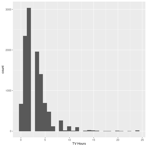
EDA - categorical
gss_cat %>% ggplot(aes(x=marital)) + geom_bar() + labs(x = "Marital Status")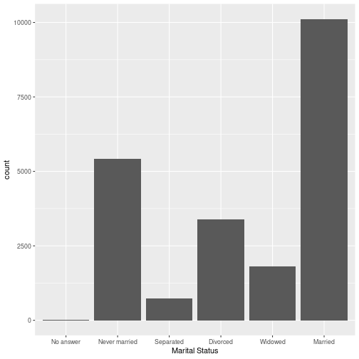
What are we trying to show?

Factors have an ordering
Factors are stored with an order even if there is no inherent meaning to the ordering
levels(gss_cat$marital)## [1] "No answer" "Never married" "Separated" "Divorced" ## [5] "Widowed" "Married"Reorder factor levels
fct_inorder(): by the order in which they first appear.
fct_infreq(): by number of observations with each level (largest first)
fct_inseq(): by numeric value of level.
https://forcats.tidyverse.org/reference/fct_inorder.html
Example
f <- factor(c("b", "b", "a", "c", "c", "c"))f## [1] b b a c c c## Levels: a b cfct_inorder(f)## [1] b b a c c c## Levels: b a cYour Turn 2
Use ggplot and one of these forcats functions to recreate the plot of gss_cat:
fct_inorder()fct_infreq()fct_inseq()

Your Turn 2 Solution
gss %>% ggplot( aes( x = fct_infreq(marital) ) ) + geom_bar() + labs(x = "Marital Status")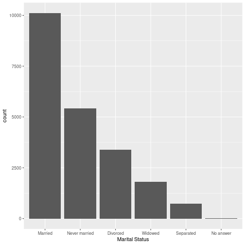
3.
Dates
Lubridate is a package that makes it easier to work dates and datetimes. These are two standard formats for storing time-related information. A date is what is sounds like - the information for a date, so the year, month, and day.
A datetime stores all of that as well as hours, minutes, seconds, and time zone.
Creating Dates and Datetimes
When working with time-related information, often the first step is to get your data into a date or datetime format.
When reading your data into R, it may be expressed in a variety of ways. The lubridate functions are built to make this transformation as intuitive and flexible as possible.
You may be trying to read in time-related information that uses dashes to separate values. Or maybe spaces, periods, or no spacing at all.
Lubridate functions will handle all of these formats automatically. A function called ymd for year/month/day can read all of these different formats and will output the Date object shown on the right.
Creating Dates and Datetimes
There are a number of functions that lubridate includes for creating a date or datetime from almost any format. Many of them are listed in this table. There are many permutations on y, m, and d, that are designed to read in time-related information that is stored in different orders.
Extract Information
Once we have our data in a date or datetime format, we are able to easily access all of the components used to build the object, such as the year, month, day, etc.
Extract Information
And, we can even extract additional information such as the quarter, week of the year, day of the year, or day of the week.
Other tasks with lubridate
do math with dates and datetimes
convert between time zones
work with time intervals
Some additional tasks that can be completed using lubridate functions are to:
do math with dates and datetimes, meaning we can add and subtract time-related information
convert between different time zones
account for leap time
round times, for example rounding dates to the nearest week or month
work with intervals of time
Bike Traffic data set
bike_traffic## # A tibble: 85,810 × 5## date crossing direction bike_count ped_count## <fct> <fct> <fct> <int> <int>## 1 02/28/2019 11:00:00 PM Burke Gilman Trail North 0 0## 2 02/28/2019 10:00:00 PM Burke Gilman Trail North 0 0## 3 02/28/2019 09:00:00 PM Burke Gilman Trail North 2 0## 4 02/28/2019 08:00:00 PM Burke Gilman Trail North 2 1## 5 02/28/2019 07:00:00 PM Burke Gilman Trail North 6 0## 6 02/28/2019 06:00:00 PM Burke Gilman Trail North 13 5## 7 02/28/2019 05:00:00 PM Burke Gilman Trail North 19 15## 8 02/28/2019 04:00:00 PM Burke Gilman Trail North 26 23## # ℹ 85,802 more rowsHere is a dataset containing bicycle traffic counts that we just loaded into R. The date column is stored as a factor with hours listed in AM and PM and is not currently in the standardized datetime format.
In the current form, we cannot take advantage of the many time-related tools that exist for dates and datetimes.
Get into a datetime format
bike_traffic %>% mutate( timestamp = mdy_hms(date, tz = "US/Pacific"), .before = date )## # A tibble: 85,810 × 6## timestamp date crossing direction bike_count ped_count## <dttm> <fct> <fct> <fct> <int> <int>## 1 2019-02-28 23:00:00 02/28/2019 11:00:… Burke G… North 0 0## 2 2019-02-28 22:00:00 02/28/2019 10:00:… Burke G… North 0 0## 3 2019-02-28 21:00:00 02/28/2019 09:00:… Burke G… North 2 0## 4 2019-02-28 20:00:00 02/28/2019 08:00:… Burke G… North 2 1## 5 2019-02-28 19:00:00 02/28/2019 07:00:… Burke G… North 6 0## # ℹ 85,805 more rowsSo, we will use a lubridate function to turn this column into a datetime.
Because our data was in the order Month-Day-Year-Hour-Minute-Second, we used the MDY_HMS function to turn the column of values into datetimes.
Your Turn 3
What day of the week was the moon landing (July 20, 1969)?
ymd(____) %>% ____(label = TRUE)Your Turn 3 Solution
What day of the week was the moon landing (July 20, 1969)?
ymd("1969-07-20") %>% wday(label = TRUE)## [1] Sun## Levels: Sun < Mon < Tue < Wed < Thu < Fri < SatNext up: Project work
Option 1: Employee Attrition project
Option 2: Explore your own data
⏰ Until coffee break (3:00 PM)